Tutorial
This tutorial shows how to perform diffusion-weighted MR simulations using Disimpy. To follow along, install the package and execute the code in each cell in the order they are presented.
💡 Google Colab is the easiest way to use Disimpy! You can use Colab to run this notebook interactively in your browser, even if you don’t have an Nvidia CUDA-capable GPU. To use a GPU on Google Colaboratory, select Runtime > Change runtime type > Hardware Type: GPU in the top menu.
[1]:
# If Disimpy has not been installed, uncomment the following line and execute
# the code in this cell

# %pip install disimpy
[2]:
# Import the packages and modules used in this tutorial

import os
import pickle
import numpy as np
import matplotlib.pyplot as plt

from disimpy import gradients, simulations, substrates, utils
Simulation parameters
We need to define the number of random walkers and diffusivity. In this tutorial, we will use a small number of random walkers to keep the simulation runtime short and to be able to quickly visualize the random walks. However, in actual experiments, a larger number of random walkers should be used to ensure that the signal converges, and the random walk trajectories do not need to be saved.
[3]:
n_walkers = int(1e3)
diffusivity = 2e-9  # SI units (m^2/s)
Gradient arrays
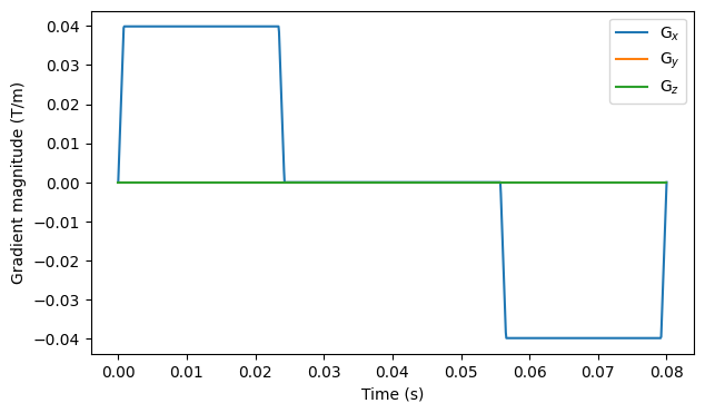
We need to define a gradient array that contains the necessary information about the simulated magnetic field gradients for diffusion encoding. Gradient arrays are numpy.ndarray instances with shape (number of measurements, number of time points, 3). The elements of gradient arrays are floating-point numbers representing the gradient magnitude along an axis at a time point in SI units (T/m). The module disimpy.gradients contains several useful functions for creating and modifying
gradient arrays. In the example below, we define a gradient array to be used in this tutorial.
[4]:
# Create a simple Stejskal-Tanner gradient waveform

gradient = np.zeros((1, 100, 3))
gradient[0, 1:30, 0] = 1
gradient[0, 70:99, 0] = -1
T = 80e-3  # Duration in seconds


# Increase the number of time points

n_t = int(1e3)  # Number of time points in the simulation
dt = T / (gradient.shape[1] - 1)  # Time step duration in seconds
gradient, dt = gradients.interpolate_gradient(gradient, dt, n_t)


# Concatenate 100 gradient arrays with different b-values together

bs = np.linspace(0, 3e9, 100)  # SI units (s/m^2)
gradient = np.concatenate([gradient for _ in bs], axis=0)
gradient = gradients.set_b(gradient, dt, bs)


# Show gradient magnitude over time for the last measurement

fig, ax = plt.subplots(1, figsize=(7, 4))
for i in range(3):
    ax.plot(np.linspace(0, T, n_t), gradient[-1, :, i])
ax.legend(["G$_x$", "G$_y$", "G$_z$"])
ax.set_xlabel("Time (s)")
ax.set_ylabel("Gradient magnitude (T/m)")
plt.show()
Substrates
We need to define the simulated diffusion environment, referred to as a substrate, by creating a substrate object. The module disimpy.substrates contains functions for creating substrate objects. Disimpy supports simulating diffusion without restrictions, in a sphere, in an infinite cylinder, in an ellipsoid, and restricted by arbitrary geometries defined by triangular meshes.
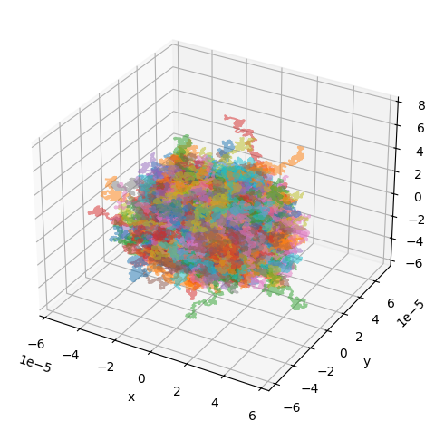
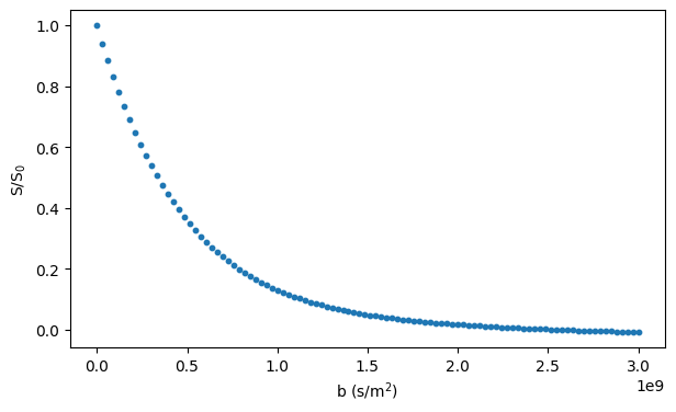
Free diffusion
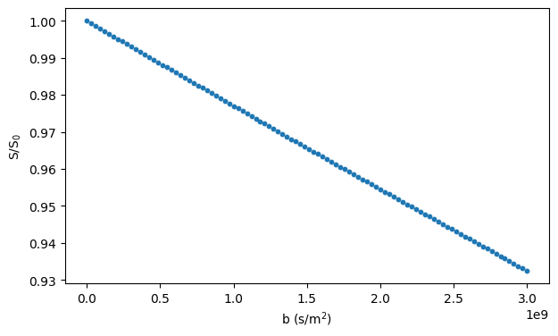
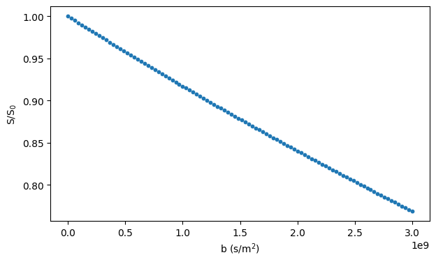
[5]:
# Create a substrate object for free diffusion
substrate = substrates.free()
# Run simulation and show the random walker trajectories
traj_file = "example_traj.txt"
signals = simulations.simulation(
n_walkers=n_walkers,
diffusivity=diffusivity,
gradient=gradient,
dt=dt,
substrate=substrate,
traj=traj_file,
)
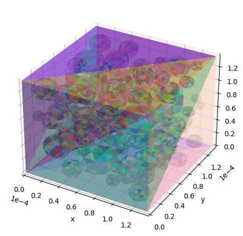
utils.show_traj(traj_file)
# Plot the simulated signal
fig, ax = plt.subplots(1, figsize=(7, 4))
ax.scatter(bs, signals / n_walkers, s=10)
ax.set_xlabel("b (s/m$^2$)")
ax.set_ylabel("S/S$_0$")
plt.show()
Starting simulation
The trajectories file will be up to 0.075 GB
Number of random walkers = 1000
Number of steps = 1000
Step length = 9.802861627917437e-07 m
Step duration = 8.008008008008008e-05 s
Simulation finished
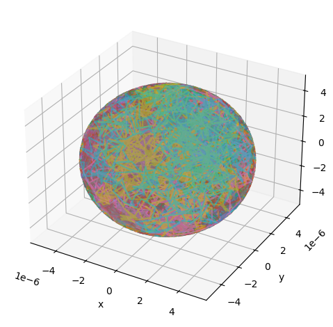
Spheres
Simulating diffusion inside a sphere requires specifying the radius of the sphere:
[6]:
# Create a substrate object for diffusion inside a sphere

substrate = substrates.sphere(radius=5e-6)


# Run simulation and show the random walker trajectories

traj_file = "example_traj.txt"
signals = simulations.simulation(
    n_walkers=n_walkers,
    diffusivity=diffusivity,
    gradient=gradient,
    dt=dt,
    substrate=substrate,
    traj=traj_file,
)
utils.show_traj(traj_file)


# Plot the simulated signal

fig, ax = plt.subplots(1, figsize=(7, 4))
ax.scatter(bs, signals / n_walkers, s=10)
ax.set_xlabel("b (s/m$^2$)")
ax.set_ylabel("S/S$_0$")
plt.show()
Starting simulation
The trajectories file will be up to 0.075 GB
Number of random walkers = 1000
Number of steps = 1000
Step length = 9.802861627917437e-07 m
Step duration = 8.008008008008008e-05 s
Simulation finished
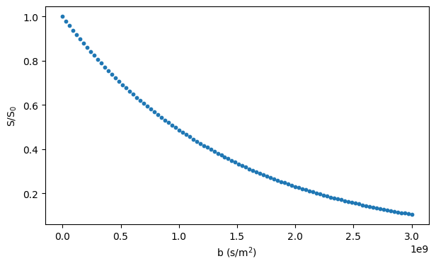
Infinite cylinder
Simulating diffusion inside an infinite cylinder requires specifying the radius and orientation of the cylinder:
[7]:
# Create a substrate object for diffusion inside an infinite cylinder

substrate = substrates.cylinder(radius=5e-6, orientation=np.array([1.0, 1.0, 1.0]))


# Run simulation and show the random walker trajectories

traj_file = "example_traj.txt"
signals = simulations.simulation(
    n_walkers=n_walkers,
    diffusivity=diffusivity,
    gradient=gradient,
    dt=dt,
    substrate=substrate,
    traj=traj_file,
)
utils.show_traj(traj_file)


# Plot the simulated signal

fig, ax = plt.subplots(1, figsize=(7, 4))
ax.scatter(bs, signals / n_walkers, s=10)
ax.set_xlabel("b (s/m$^2$)")
ax.set_ylabel("S/S$_0$")
plt.show()
Starting simulation
The trajectories file will be up to 0.075 GB
Number of random walkers = 1000
Number of steps = 1000
Step length = 9.802861627917437e-07 m
Step duration = 8.008008008008008e-05 s
Simulation finished
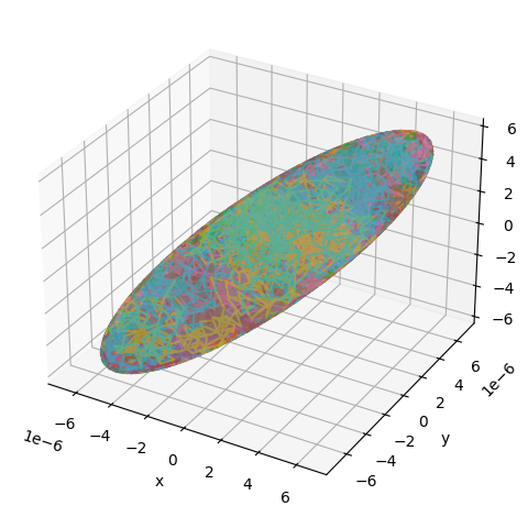
Ellipsoids
Simulating diffusion inside an ellipsoid requires specifying the ellipsoid semiaxes and a rotation matrix, defining the ellipsoid orientation, according to which the axis-aligned ellipsoid is rotated before the simulation:
[8]:
# Create a substrate object for diffusion inside an ellipsoid

v = np.array([1.0, 0, 0])
k = np.array([1.0, 1.0, 1.0])
R = utils.vec2vec_rotmat(v, k)  # Rotation matrix for aligning v with k
substrate = substrates.ellipsoid(
    semiaxes=np.array([10e-6, 5e-6, 2.5e-6]),
    R=R,
)


# Run simulation and show the random walker trajectories

traj_file = "example_traj.txt"
signals = simulations.simulation(
    n_walkers=n_walkers,
    diffusivity=diffusivity,
    gradient=gradient,
    dt=dt,
    substrate=substrate,
    traj=traj_file,
)
utils.show_traj(traj_file)


# Plot the simulated signal

fig, ax = plt.subplots(1, figsize=(7, 4))
ax.scatter(bs, signals / n_walkers, s=10)
ax.set_xlabel("b (s/m$^2$)")
ax.set_ylabel("S/S$_0$")
plt.show()
Starting simulation
The trajectories file will be up to 0.075 GB
Number of random walkers = 1000
Number of steps = 1000
Step length = 9.802861627917437e-07 m
Step duration = 8.008008008008008e-05 s
Simulation finished
Triangular meshes
Diffusion restricted by arbitrary geometries can be simulated using triangular meshes.
Triangular meshes must be represented by a pair of numpy.ndarray instances: vertices array with shape (number of points, 3) containing the points of the triangular mesh, and faces array with shape (number of triangles, 3) defining how the triangles are made up of the vertices. The simulated voxel is equal to the axis-aligned bounding box of the triangles plus optional padding. Before the simulation, the triangles are moved so that the bottom corner of the simulated voxel is at the origin.
By default, the initial positions of the random walkers are randomly sampled from a uniform distribution over the simulated voxel. If the triangles define a closed surface, the initial positions of the random walkers can be randomly sampled from a uniform distribution over the volume inside or outside the surface. For very complex meshes, the current implementation of the algorithm that samples positions inside or outside the surface may require changes to the code. The initial positions can also be defined manually.
Disimpy supports periodic and reflective boundary conditions. If periodic boundary conditions are used, the random walkers encounter infinitely repeating identical copies of the simulated microstructure after they leave the simulated voxel. Otherwise, the boundaries of the simulated voxel are treated as impermeable surfaces.
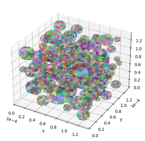
The code below loads an example mesh and shows how to generate a substrate object for simulating diffusion inside the closed surface.
[9]:
# Load an example triangular mesh
mesh_path = os.path.join(
os.path.dirname(simulations.__file__), "tests", "example_mesh.pkl"
)
with open(mesh_path, "rb") as f:
example_mesh = pickle.load(f)
faces = example_mesh["faces"]
vertices = example_mesh["vertices"]
# Create a substrate object
substrate = substrates.mesh(
vertices, faces, padding=np.zeros(3), periodic=True, init_pos="intra"
)
# Show the mesh
utils.show_mesh(substrate)
# Run simulation and show the random walker trajectories
traj_file = "example_traj.txt"
signals = simulations.simulation(
n_walkers=n_walkers,
diffusivity=diffusivity,
gradient=gradient,
dt=dt,
substrate=substrate,
traj=traj_file,
)
utils.show_traj(traj_file)
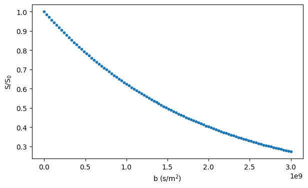
# Plot the simulated signal
fig, ax = plt.subplots(1, figsize=(7, 4))
ax.scatter(bs, signals / n_walkers, s=10)
ax.set_xlabel("b (s/m$^2$)")
ax.set_ylabel("S/S$_0$")
plt.show()
Aligning the corner of the simulated voxel with the origin
Moved the vertices by [0. 0. 0.]
Dividing the mesh into subvoxels
Finished dividing the mesh into subvoxels
Starting simulation
The trajectories file will be up to 0.075 GB
Number of random walkers = 1000
Number of steps = 1000
Step length = 9.802861627917437e-07 m
Step duration = 8.008008008008008e-05 s
Calculating initial positions
Finished calculating initial positions
Simulation finished
[10]:
# Create and show a substrate object with reflective boundary conditions

substrate = substrates.mesh(
    vertices, faces, padding=np.zeros(3), periodic=False, init_pos="intra"
)
utils.show_mesh(substrate)
Aligning the corner of the simulated voxel with the origin
Moved the vertices by [0. 0. 0.]
Dividing the mesh into subvoxels
Finished dividing the mesh into subvoxels
Importing mesh files
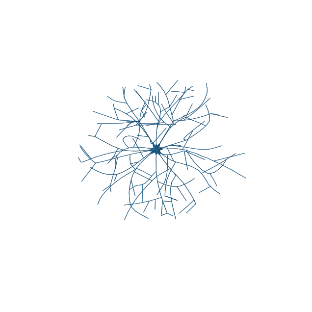
There are several open-source Python packages for reading mesh files. The code snippet below shows how to use meshio to load a mesh of a neuron model generated using an algorithm by Palombo et al.
[11]:
# If meshio has not been installed, uncomment the following line and execute
# the code in this cell

# %pip install meshio>=5.3.5
import meshio


# Load mesh

mesh_path = os.path.join(
    os.path.dirname(simulations.__file__), "tests", "neuron-model.stl"
)
mesh = meshio.read(mesh_path)
vertices = mesh.points.astype(np.float32)
faces = mesh.cells[0].data


# Show mesh using Matplotlib's trisurf

fig = plt.figure(figsize=(8, 8))
ax = fig.add_subplot(111, projection="3d")
ax.plot_trisurf(
    vertices[:, 0],
    vertices[:, 1],
    vertices[:, 2],
    triangles=faces,
)
plt.axis("off")
plt.show()
Advanced information
For details, please see the reference and source code. More information about a function can be found in the docstrings. For example,
[12]:
simulations.simulation?
Signature:
simulations.simulation(
    n_walkers,
    diffusivity,
    gradient,
    dt,
    substrate,
    seed=123,
    traj=None,
    final_pos=False,
    all_signals=False,
    quiet=False,
    cuda_bs=128,
    max_iter=1000,
    epsilon=1e-13,
)
Docstring:
Simulate a diffusion-weighted MR experiment and generate signal. For a
detailed tutorial, please see
https://disimpy.readthedocs.io/en/latest/tutorial.html.

Parameters
----------
n_walkers : int
    Number of random walkers.
diffusivity : float
    Diffusivity in SI units (m^2/s).
gradient : numpy.ndarray
    Floating-point array of shape (number of measurements, number of time
    points, 3). Array elements represent the gradient magnitude at a time
    point along an axis in SI units (T/m).
dt : float
    Duration of a time step in the gradient array in SI units (s).
substrate : disimpy.substrates._Substrate
    Substrate object containing information about the simulated
    microstructure.
seed : int, optional
    Seed for pseudorandom number generation.
traj : str, optional
    Path of a file in which to save the simulated random walker
    trajectories. The file can become very large! Every line represents a
    time point. Every line contains the positions as follows: walker_1_x
    walker_1_y walker_1_z walker_2_x walker_2_y walker_2_z…
final_pos : bool, optional
    If True, the signal and the final positions of the random walkers are
    returned as a tuple.
all_signals : bool, optional
    If True, the signal from each random walker is returned instead of the
    total signal.
quiet : bool, optional
    If True, updates on the progress of the simulation are not printed.
cuda_bs : int, optional
    The size of the one-dimensional CUDA thread block.
max_iter : int, optional
    The maximum number of iterations allowed in the algorithm that checks
    if a random walker collides with a surface during a time step.
epsilon : float, optional
    The amount by which a random walker is moved away from the surface
    after a collision to avoid placing it in the surface.

Returns
-------
signal : numpy.ndarray
    Simulated signals.
File:      ~/disimpy/disimpy/simulations.py
Type:      function
For details, please see the reference and source code.